Machine learning is a scientific practice which is heavily tied with the terms “error” and “approximation”. Sciences like Mathematics and Physics are associated with error, induced by a need to model how things work. Moreover, the abilities of humans in intelligence tasks are also tied with error, since some actions associated with these abilities may be the result of failure, while other actions may be deemed as truly successful ones. There have been myriads of times when our thinking, our categorization ability, or our human decisions, have failed. Machine learning models, which try to mimic and compete with human intelligence in certain tasks, are also tied with successful operations or erroneous ones.
But how can a machine learning model, a deterministic model with the ability to empirically compute the confidence it has for a particular action, diagnose itself that it makes an error when processing a particular input? Even for a machine learning engineer, trying to intuitively understand why without studying a particular method seems difficult.
In this article, we discuss a recent algorithm for this problem that convincingly explains how; in particular, we describe the Language Based Error Explainability (LBEE) method by Csurka et al. Here, we will recreate an explanation on how this method leverages the convenience of generating embeddings via the CLIP model contributed by OpenAI, which allows one to translate text extracts and images into high-dimensional vectors that reside in a common vector space. By projecting texts or images in this common high-dimensional space, we can compute the dot product between two embeddings (which is a well-known operation that measures the similarity among two vectors) to quantitatively measure how similar the two original text/image objects are as a function of other dot product operations (or, put simply, other similarities among vectors) involving pairs of other objects.
The designers of LBEE have developed a model that can report a textual error description of a model failure in cases where the underlying model asserts an empirically low confidence score in taking an action that the model was designed for. Part of the difficulty in grasping how such a method fundamentally works is our innate wondering about how the textual descriptions explaining the model failure are generated from scratch as a function of an input datum. In our brains, we often do not put much effort when we need to explain why a failure happens and we instantly arrive at clues to describe them, unless the cause drifts apart from our fundamental understanding of the inner workings of the object that is involved in the failure. To keep things interesting, we can provide an answer to this wondering: instead of assembling these descriptions once for each input, we can generate them following a recipe a-priori and then reuse them in the LBEE task by computationally reasoning about the relevance of a candidate set of explanations in relation to a given model input. In the remainder of this article, we will see how:
Suppose that we have a classification model that was trained to classify the object type of an only object depicted in a small color image. We could, for example, take photographs of objects in a white background with our phone camera and pass these images to the model in order for it to classify the object names. The classification model can yield a confidence score ω that is between 0 and 1, representing the normalized confidence that the model has when assigning the images to a particular class in relation to all the possible object types that are recognizable by the model. It is usually observed that when a model does poorly in generating a prediction, the resulting confidence score may be quite low. But what is a good empirical threshold T that allows us to identify a poor prediction or a confident prediction? To empirically estimate two such thresholds, one for identifying easy predictions and one for identifying hard predictions, we can take a large dataset of images (e.g., the ImageNet datase) and pass each image to the classifier. For the images which were classified correctly, we can plot the confidence scores generated by the model as a normalized histogram. By doing so, we may expect to see two large lobes in the histogram, representing the confidence values which correspond to confident inferences and less confident inferences. We may also expect to see some degradation in the frequency masses around the two lobes, which is possible. Otherwise, we would come up with a histogram presenting two lobes which are highly leptokurtic. One lobe concentrates empirical prediction scores that are lower, and a second lobe will concentrate many scores which are relatively high. Then, we can set an empirical threshold that separates the two lobes.

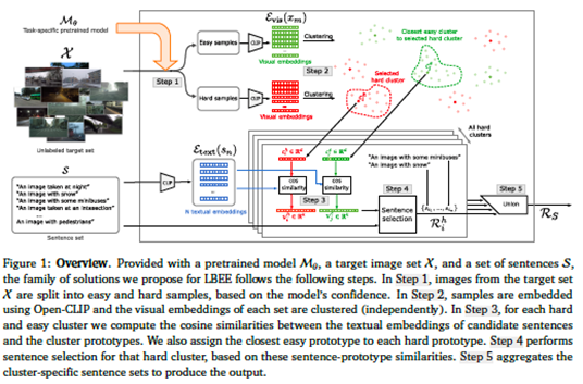
Csurka and collaborators designate separating images as easy or hard based on the confidence score of a classification machine learning model and their relation to the cut-off threshold (see Figure 1). By distinguishing these two image sets, the authors compute the embeddings of the images from each group, and for each image in these sets they compute an ordered sequence of numbers (for our convenience, we will use the term vector to refer to this sequence of numbers) which describe the semantic information of the image. To do this, they employ the CLIP model contributed by OpenAI, the company that is famous for the delivery of the ChatGTP chatbot model, which excels at producing embeddings for images and text in a joint high-dimensional vector space. The computed embeddings can be used to measure the similarity between an image and a very small text extract, or the similarity between a pair of text extracts or images.
As a later step, the authors wanted to identify the groups of image embeddings that share similarities. To do this, they use a clustering algorithm which can take in vectors generated by a “generating machine” and identify the clusters of the embeddings. The number of clusters that fit a particular dataset is non-trivial to define. All in all, we come up with two types of clusters: clusters of CLIP embeddings for “easy” images, and clusters of CLIP embeddings for “hard” images. Then, any hard cluster center is picked and for it the closest easy cluster center is found. This allows us coming up with two embedding vectors originating from the clustering algorithm. The two clusters, “easy” and “hard”, are visually denoted at the top-right sector of Figure 1, by green and red -dotted enclosures.
The LBEE algorithm then generates a set S of sentences that describe the above-said images. Therefore, for each short sentence that is generated, the CLIP embedding is computed. As it was mentioned earlier, this text embedding can be directly compared to the embedding of any image by calculating the dot product (or inner product) of the two embedding vectors. Consider that the dot product measures a quantity that in the signal processing community is called linear correlation. The authors apply this operation directly. They compute the similarity of each text error description by computing the so-called cosine similarity measure between a text extract embedding and an image embedding, ultimately computing two relevance score vectors of dimensionality k < N. Each dimension is tied with a given textual description. By taking these two score vectors into consideration, the authors pass the two vectors in a sentence selection algorithm (we cover them in the next paragraph). The selected sentences are considered for this forward process by taking into account each hard cluster. The union of these sentence-sets is then output to the user, in return for an image that was supplied as input.

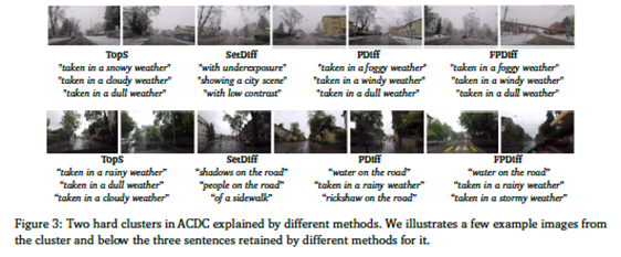
The authors chose to define four sentence selection algorithms, named SetDiff, PDiff, FPDiff and TopS. SetDiff computes the sentence-sets corresponding to a hard cluster and to an easy cluster. Then, the algorithm removes from the hard cluster sentence-set the sentences that also appear in the easy cluster sentence-set, and reports the resulting set to the user. PDiff takes two similarity score vectors i and j of dimensionality $k$ (where k denotes the top-$k$ relevant text descriptions), one from the hard set and one from the easy set. Then, Diff computes the difference between these two vectors, and from there it retains the sentences corresponding to the top $k$ values. TopS trivially reports as an answer all the sentences that correspond to the vector of top-k similarities. Figure 3 presents an example of textual failure modes generated by a computer vision model, each using one of the TopS, SetDiff, Diff and FPDiff methods. To enable evaluation of the LBEE model and methodology, the authors had to also introduce an auxiliary set of metrics, adapted to the specificalities of the technique. To further understanding on this innovative and very useful work, we recommend you to keep on reading [1].
References
[1] What could go wrong? Discovering and describing failure modes in computer vision, published in the proceedings of ECCV 2024.
Sotiris Karavarsamis
Research Assistant at Visual Computing Lab (VCL)@CERTH/ITI

